- Fourier Transform
- Common Functions
- Sampling
- Correlation
- Wave separation
-
Seismic applications
- Introduction Seismic applications
- Processing of a shot point
- Dispersion analysis of Rayleigh waves
- Love Waves
- Refraction - Reflection seismic survey
- Seismic processing with an industrial software
- Processing of a 3D shot point
- VSP processing
- Marine vibrator
- Multi component OBS
- Dispersion Analysis with OBS data
- Rayleigh waves: f-k filtering
- Rayleigh waves: dispersion analysis
- Rayleigh waves: SVD filtering
- Rayleigh waves: SMF filtering
-
The Hilbert transformation
- Introduction The Hilbert transformation
- Hilbert transform and envelope computation
- Hilbert transform and phase change
- Hilbert transform and instantaneous frequency
- Hilbert transform and analytic signal
- Hilbert transform and polarization
- Polarization filter
- Measurement of group and phase velocities
- Zero phase georadar section
-
Filtering
- Introduction Filtering
- Boxcar filters
- a first order MA filter
- a first order AR filter
- a second order MA filter
- a second order AR filter
- a Butterworth ARMA filter
- Inverse filter
- AR2 inverse filter
- Wiener filter: spiking deconvolution
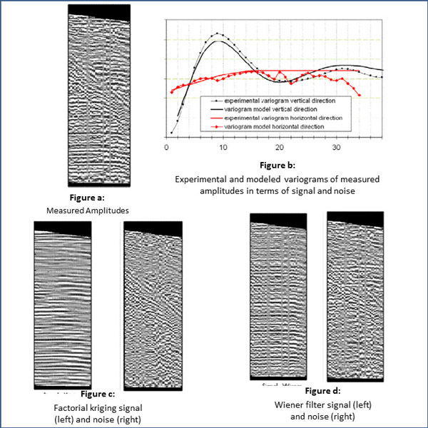
- Wiener filter: Study of the variability of a seismic section
- Wiener filter: predictive deconvolution
-
Near Surface Geophysics
- Introduction Near Surface Geophysics
- 3D seismic survey
- 3C VSP at well C1
- VSP with a hydrophone at well C1
- VSP with a hydrophone at well M3
- VSP with a hydrophone at well M20
- Acoustic logging at well M20
- Flows
- 3D Imaging
- VSP and depth conversion
- Acoustic logging and cementing
- Calibration and Synthetic seismograms
- Stochastic Signal Processing
- Attributes


