Stochastic modeling enables consistent integration of all sources of time to depth conversion uncertainties within a unique probability (or “stochastic”) model. From a mathematical standpoint, the stochastic time to depth conversion model guarantees unbiased estimations of depth, interval velocities, thicknesses, and volumes, as well as realistic confidence intervals (P10, P50, P90 values).

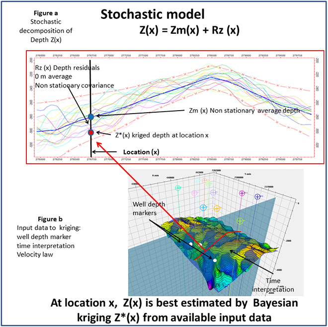
In essence, the stochastic time to depth conversion model is non-stationary and induces complex variance and co-variance computations. Unknown depth Z at location x is expressed as the sum of the depth “trend” Zm and depth “residuals” Rz (please see Figure a):

• Zm corresponds to the non-stationary average or spatial “trend” of Z, derived from interpreted time maps and prior velocity model + associated parameters (e.g. V0, K etc.)
• Rz corresponds to residual depth fluctuations around Zm, derived from uncertainty on time interpretations, interval velocities and prior velocity model + associated parameters.

• As shown in Formulas, Rz has a non-stationary covariance C(x,y).

Once the variance and covariance models are defined (see Formulas), depth estimation using kriging becomes straightforward. The most adapted kriging operator is Bayesian Kriging (Omre et al 1987). The approach exposed in this course is inspired by Abrahamsen’s multilayer stochastic depth conversion case (Abrahamsen P. 1993) and extended to non-linear depth trend functions derived from different velocity models.

As an end result, the Bayesian co-kriging algorithm best estimates the depth trend parameters and the depth tying residuals at the well locations (please see Figure b). It ensures that, for all horizons simultaneously, kriged depth trend parameters lead to 0m centered and minimum variance kriged depth residuals.