Chapter 2:
From Fundamental to Properties

Abstract

List of examples

Example 2.7: Distillation column

A mixture of light hydrocarbons is processed in a distillation column. Compositions of distillate obtained from the total condenser and of the residue at the bottom of the column are as follows (see figure 1):

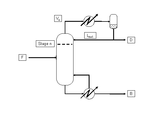Figure 1: VL equilibria in a distillation column

Table 1: Distillate and residue composition for example

Component	Distillate	Residue
Propane	0.23
iso-Butane	0.67	0.02
n-Butane	0.10	0.46
iso-Pentane		0.15
n-Pentane		0.37

a) What is the column pressure to obtain the specified distillate if temperature in the condenser drum is 120 °F? (The pressure drop in column, exchanger and drum will be neglected.)
b) What is the temperature in the upper stage and the composition of the liquid pouring off this plate (number n on the figure)?
c) What is the temperature in the reboiler?

Use the Scheibel and Jenny diagram (Figure 2) to evaluate the distribution coefficients.

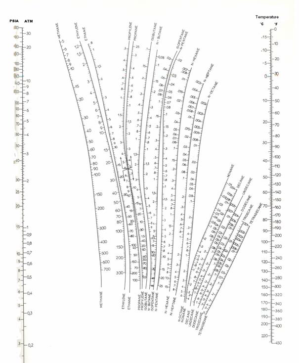Figure 2: Scheibel and Jenny nomograph for light hydrocarbons.

Analysis:

a) In the condenser, the liquid composition is known. Since a liquid equilibrium with a vapour is at its bubble point, the pressure is the bubble pressure. The pressure is a constant in the column.
b) The overall mass balance around the condenser indicates that all flows have the same composition. Hence, the vapour leaving the top plate of the column has the distillate composition. In addition, this vapour is saturated and is therefore at its dew point. As pressure is known (calculated in a), temperature has to be computed (dew temperature) and liquid composition will be a part of the answer.
c) The residue from the reboiler is also a liquid phase. Pressure is unchanged, so bubble temperature must be calculated.

Components are all light hydrocarbons and we are told to use the Scheibel and Jenny procedure. This procedure assumes an ideal mixture (equilibrium coefficients are independent of composition) and is more suitable than Raoult's law at expected working pressure (10 bar).

All calculations are relative to vapour-liquid equilibrium and none of the HC in the mixture is at supercritical conditions.

Solution:

See complete results in file (xls):

Download

Some help on nomenclature and tips to use this file can be found here.

a) A bubble pressure is calculated using . In order to be able to read the equilibrium constant (Ki) in the Scheibel and Jenny diagram, both pressure and temperature are needed. A first pressure must be guessed, so distribution coefficients can be read on the monograph. Raoult's law can be used as a first approximation: The estimated pressure is 8.5 atm.
Now, a new line must be drawn between the point T = 120 °F and P = 8.5 atm. The three Ki are read on the figure 2. On the first attempt, the sum is not equal to 1 (see table 2). A different guess must be made (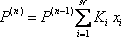). Due to the poor accuracy of the graphical method, the result can be considered to be reached in the second iteration. The bubble point of the mixture is 8.4 atm. The procedure is summarized in table 2.

Table 2 Results of bubble pressure computing

Component
Propane	0.23	16.5	1.68	0.387	1.70	0.391
iso-Butane	0.67	6.3	0.81	0.543	0.82	0.594
n-Butane	0.10	4.6	0.62	0.062	0.62	0.062

Sum/Result		8.48		0.991		1.002

b) Since the pressure drop is neglected, the entire column is assumed to be at 8.4 atm. We will start the calculation with the same value for the distribution coefficients. A dew point is calculated and the criteria must be satisfied. At the first iteration (table 3), as the composition of the liquid phase is not correct (sum equal to 1.11), the composition is normalised, allowing us to calculate a hypothetical iso-butane distribution coefficient (K3=0.67/0.734=0.91). A line is drawn at the same pressure through this point and the other values of are read and introduced in the table. Convergence is reached in almost two iterations, with a final temperature of 132 °F as summarized in table 3.

Table 3: Results of example of the dew temperature

Component
Propane	0.23	1.7	0.14	0.12	1.85	0.12
iso-Butane	0.67	0.82	0.82	0.73	0.91*	0.73
n-Butane	0.10	0.26	0.16	0.14	0.72	0.14

Sum/Result			1.11			1.00

* calculated using (K=0.67/0.73=0.91)

c) The reboiler is the equipement where liquid at the bottom of the column exits the system while vapour in equilibrium is reinjected. This is a new bubble point problem where the pressure is known, and the temperature is to be calculated. In this case again, convergence is reached when .
After the first iteration (table 4), the vapour composition is normalised and a K (in this case n-butane is used) is estimated. The line is drawn through this value and the pressure of the column. In this case, two different iterations are necessary. The distribution coefficients are given for the two intermediate calculations and the final result.

Table 4: Composition of reboiler


iC4	0.02	0.91	0.018	0.037	1.78	1.70	0.034
nC4	0.46	0.72	0.331	0.671	1.46*	1.37	0.629
iC5	0.15	0.32	0.048	0.097	0.77	0.74	0.111
nC5	0.37	0.26	0.096	0.195	0.66	0.63	0.233

Sum/			0.493	1.000			1.007

* calculated using (K=0.67/0.46 = 1.46)

The temperature of the reboiler is found to be 197°F.

Chapter 2: From Fundamental to Properties