Chapter 3:
From Components
to Models
Abstract
Read the abstractTable of contents
See the table of contentsList of examples
- 3-1: Vapour pressure predictions of methane using different formulas
- 3-2: Quality evaluation of molar volume correlations
- 3-3: Evaluation of the ideal gas heat capacity equations for n-pentane
- 3-4: Quality evaluation of vapourisation enthalpy correlations
- 3-5: Comparison of second virial coefficient calculation methods
- 3-6: Comparison of critical points and acentric factor from different databases
- 3-7: Use of the group contribution methods of Joback and Gani
- 3.8: Diesel fuel characterization
- 3.9: Vapour pressures of di-alcohols
- 3.10: Find the parameters to fit the vapour pressure of ethyl oleate
- 3.11: Fitting of BIP coefficients for the mixture water + MEA with the NRTL model
- 3.12: Separation of n-butane from 1,3 butadiene at 333.15K using vapour-liquid equilibrium
- 3.13: Draw the heteroazeotropic isothermal phase diagram of the binary mixture of water and butanol at 373.15 K
- 3.14: Isothermal phase diagram using the Flory Huggins activity coefficient model
- 3.15: Use of an equation of state for pure component vapour pressure calculations
Example 3-5: Comparison of second virial coefficient calculation methods
A comparison of second virial coefficient for hydrocarbon is to be proposed. Differences between different correlations will be analysed. The various equations are the following:
DIPPR form:

Tsonopoulos form:

where

Ambrose form:

In these relationships, the reduced temperature is defined as: . Coefficients for the different equations are:
| Tc (K) | Pc (kPa) | ω |
|---|---|---|
| 562.05 | 4895 | 0.2212 |
| Equation | A | B | C | D | E | Tmin.(K) | Tmax(K) |
|---|---|---|---|---|---|---|---|
| DIPPR | 0.1509 | -186.94 | -2.3146.107 | -7.05.1018 | -6.88.1022 | 281 | 1500 |
| Ambrose | 571.4 | -348.4 | 526.6 | - | - | 290 | 600 |
| Tsonopoulos | From critical parameters | 281 | 1500 | ||||
Analysis:
- The properties are temperature and second virial coefficient.
- Component is benzene, which is a databank component.
Solution:
See complete results in file (xls):
Some help on nomenclature and tips to use this file can be found here.
A graph is constructed with the different equations: DIPPR, Tsonopoulos and Ambrose. The two former relations cover a large temperature range [281 – 1500 K], but the latter is related to a shorter temperature range and we have also extrapolated it to high temperature.
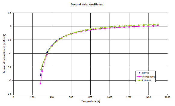 Figure 1: Second virial coefficient of benzene as a function of temperature. The Ambrose correlation has been extrapolated to high temperatures.
We have determined the Boyle’s temperature where the second virial coefficient is zero. Table 3 gives the values obtained from the three correlations.
| Correlations | Boyle’s Temperature (K) |
|---|---|
| DIPPR form | 1327.11 |
| Tsonopoulos form | 1313.84 |
| Ambrose form | 1059.64 |
We can observe that the DIPPR and the Tsonopoulos forms are in agreement with a relative difference close to 1 %. This is not the cas with the Ambrose form, which is extrapolated, we obtain a lower Boyle’s temperature (less than 255 K). This example illustrates the risk of extrapolation outside of the defined temperature range of the correlation.
References
R. L. Rowley, W. V. Wilding, J. L. Oscarson, Y. Yang, N. A. Zundel, T. E. Daubert, R. P. Danner, DIPPR® Data Compilation of Pure Compound Properties, Design Institute for Physical Properties, AIChE, New York, NY (2003).