Chapter 3:
From Components
to Models
Abstract
Read the abstractTable of contents
See the table of contentsList of examples
- 3-1: Vapour pressure predictions of methane using different formulas
- 3-2: Quality evaluation of molar volume correlations
- 3-3: Evaluation of the ideal gas heat capacity equations for n-pentane
- 3-4: Quality evaluation of vapourisation enthalpy correlations
- 3-5: Comparison of second virial coefficient calculation methods
- 3-6: Comparison of critical points and acentric factor from different databases
- 3-7: Use of the group contribution methods of Joback and Gani
- 3.8: Diesel fuel characterization
- 3.9: Vapour pressures of di-alcohols
- 3.10: Find the parameters to fit the vapour pressure of ethyl oleate
- 3.11: Fitting of BIP coefficients for the mixture water + MEA with the NRTL model
- 3.12: Separation of n-butane from 1,3 butadiene at 333.15K using vapour-liquid equilibrium
- 3.13: Draw the heteroazeotropic isothermal phase diagram of the binary mixture of water and butanol at 373.15 K
- 3.14: Isothermal phase diagram using the Flory Huggins activity coefficient model
- 3.15: Use of an equation of state for pure component vapour pressure calculations
Example 3-6: Comparison of critical points an acentric factor from different databases
This example shows comparisons of critical data between different databanks. The suggested comparison is caring in two steps. The first one is a direct comparison between the values extracted from databases. The second step discusses the impact of these differences on one of the most important property for vapour - liquid equilibrium: the vapour pressure. This example works on three hydrocarbons: vinylacetylene, 2-methyl-1-butene, trans 1,3-pentadiene. The critical temperatures and pressures and the acentric factors of two databases are given in table 1.
| Database | Vinylacetylene | 2-methyl-1-butene | Trans 1,3-Pentadiene | |
|---|---|---|---|---|
| DIPPR | Tc (K) | 454 | 465 | 500 |
| Pc (kPa) | 4860 | 3447 | 3740 | |
| ω (-) | 0.1069 | 0.2341 | 0.1162 | |
| Process Simulation Package | Tc (K) | 455.15 | 470.15 | 496.15 |
| Pc (kPa) | 4894 | 3850 | 3992 | |
| ω (-) | 0.1205 | 0.234 | 0.1719 | |
Analysis:
The properties are critical temperature, critical pressure and acentric factor.
The vapour pressure is estimated with the Lee and Kesler equation (section 3.1.1.2) which is function of critical parameters and acentric factors.
Components are hydrocarbons, which are databank components.
Solution:
See complete results in file (xls):
Some help on nomenclature and tips to use this file can be found here.
Table 2 gives the direct comparison between these values. We can observe that the critical temperature shows the lower deviation. In other hand, there is a large dispersion about the acentric factor. This kind of behaviour is common when there is a direct comparison of different sources. Generally, light compounds have similar values in different Process Simulators, but heavy compounds or branched isomers, which are less characterised, can show larger deviations. It is important to bear in mind that some published values in databases are not experimental values. Some are predicted or extrapolated. For example, the critical point is not always measurable due to cracking phenomena. The acentric factor is evaluated at reduced temperature equal to 0.7 but what is this temperature if the critical point is unknown?
| Vinylacetylene | 2-methyl-1-butene | Trans 1,3-Pentadiene | |
|---|---|---|---|
| Tc (K) | 1.15 (0.3 %) | -5.15 (1.1 %) | 3.85 (0.8 %) |
| Pc (kPa) | -34 (0.7 %) | -403 (11.7%) | -252 (6.7 %) |
| ω (-) | -0.0137 (12.8 %) | 0.0001 (0.03 %) | -0.0557 (48 %) |
However, the direct comparison of these critical values is not the best criteria to check the validation of the databank. It is important to check the sensitivity of the complete model to evaluate how much the result is affected by a small deviation of the input. As an example, the critical point and the acentric factor are generally used in order to calculate the vapour pressure.
Using any corresponding states relationship (e.g. the Lee and Kesler or the Ambrose relationship, discussed in exercise 3.1), we can calculate the vapour pressure of the three compounds as a function of temperature in the temperature range of 0.5 to 1.0 in terms of reduced temperature. The relative deviations using these two databanks parameters are the following:
- 4.9 % for the vinylacetylene;
- 2.4 % for the 2-methyl-1-butene;
- 7.7 % for the trans 1,3-Pentadiene
They are plotted in figure 1, for the example of vinylacetylene, and for both correlations.
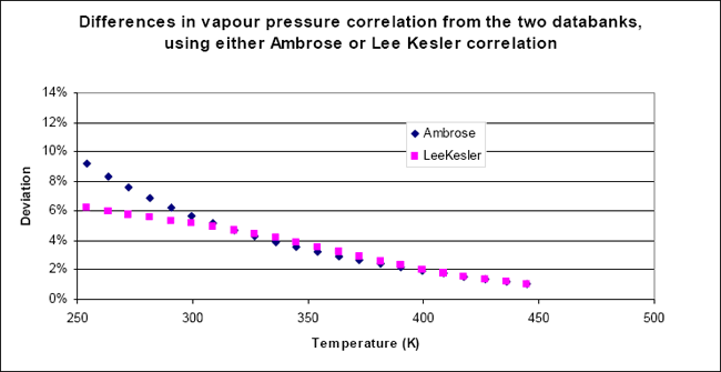 Figure 1: Differences between the predicted vapour pressures for vinylacetylene as a function of temperature, using the two databanks.
Two observations can be made, at this point:
- For any of the two correlations, the difference between the results for the two databases is small at high temperature. This is explained because for this component, the critical point parameters are very close, only the acentric factor shows a big difference, explaining why the deviation becomes large at lower temperatures
- The difference between the Lee-Kesler and the Ambrose correlations is essentially visible at low temperature. This has already been shown in exercice 3.1, where it was concluded that the Ambrose relationship extrapolates better to lower temperatures. Hence, the low temperature deviations are better evaluated using the Ambrose correlation.
To validate a databank, it is important to compare the model to experimental data. Figure 2 shows the deviation between the Ambrose correlation results and the experimental data, using both databases.
 Figure 2: Deviation between the corresponding state predictions using the DIPPR and the PROCESS database with the Ambrose correlation, and the experimental data, for 2-methyl-1-butene.
From this type of plot, it is possible to evaluate the trends of the curves with respect to temperature: the DIPPR parameters will result in smaller average deviations in the temperature range surrounding 350K, but the extrapolation towards lower temperatures will not be guaranteed. In opposition, the PROCESS database provides overall an overestimation of the vapour pressure, but the tendency with temperature is probably more acceptable.
The main conclusion of this example is that the user must not place blind trust in a value simply because it is published in a database. In addition, it should keep in mind that process simulators have generally more than one databank, and for compatibility reasons, the older database is often the default one. It is important to compare different sources of information if they are available. If a predictive model is used to calculate a property, the physical meaning of the result must be compared with known trends or behaviour.
References
R. L. Rowley, W. V. Wilding, J. L. Oscarson, Y. Yang, N. A. Zundel, T. E. Daubert, R. P. Danner, DIPPR® Data Compilation of Pure Compound Properties, Design Institute for Physical Properties, AIChE, New York, NY (2003).