Chapter 3:
From Components
to Models
Abstract
Read the abstractTable of contents
See the table of contentsList of examples
- 3-1: Vapour pressure predictions of methane using different formulas
- 3-2: Quality evaluation of molar volume correlations
- 3-3: Evaluation of the ideal gas heat capacity equations for n-pentane
- 3-4: Quality evaluation of vapourisation enthalpy correlations
- 3-5: Comparison of second virial coefficient calculation methods
- 3-6: Comparison of critical points and acentric factor from different databases
- 3-7: Use of the group contribution methods of Joback and Gani
- 3.8: Diesel fuel characterization
- 3.9: Vapour pressures of di-alcohols
- 3.10: Find the parameters to fit the vapour pressure of ethyl oleate
- 3.11: Fitting of BIP coefficients for the mixture water + MEA with the NRTL model
- 3.12: Separation of n-butane from 1,3 butadiene at 333.15K using vapour-liquid equilibrium
- 3.13: Draw the heteroazeotropic isothermal phase diagram of the binary mixture of water and butanol at 373.15 K
- 3.14: Isothermal phase diagram using the Flory Huggins activity coefficient model
- 3.15: Use of an equation of state for pure component vapour pressure calculations
Example 3-8: Diesel fuel characterization
A diesel fuel has been characterised in laboratory by a TBP curve, as shown in table 1. Its average specific gravity is given as 0.8113. For simulation purposes, this diesel must be split in 10 °C cuts.
- Find the volume percentage corresponding to each cut.
- Provide the characteristic (critical) parameters for each cut.
| Fraction distillate | 0 | 3 | 7 | 17 | 29 | 40 | 50 | 59 |
|---|---|---|---|---|---|---|---|---|
| Boiling temperature ( °C) | 123 | 162 | 185 | 206 | 226 | 244 | 262 | 279 |
| Fraction distillate | 67 | 73 | 80 | 85 | 88 | 92 | 100 | |
| Boiling temperature ( °C) | 295 | 309 | 324 | 338 | 350 | 362 | 375 |
Analysis:
The properties given are the boiling temperature as a function of fraction.
Components are a mixture of a large number of components and will be evaluated as pseudo-components.
Phases are vapour and liquid at atmospheric pressure.
Solution:
See complete results in file (xls):
Some help on nomenclature and tips to use this file can be found here.
In a first step, the cut procedure is illustrated:
The curve is obtained by an interpolation method. One of the best choices is to use a cubic spline interpolation. Once the natural condition for extrapolation is chosen, the solution of the linear system gives all the curvatures at all points (table 2). This information is used to calculate the coefficients of each cubic polynomial.
The cuts are constructed on a 10 °C width basis which requires an inverse interpolation. An iterative procedure must be implemented. The volume percent corresponding to each cut is given in the table 2 and in figure 1.
| Cut | 123-133 | 133-143 | 143-153 | 153-163 | 163-173 | 173-183 | 183-193 | 193-203 |
|---|---|---|---|---|---|---|---|---|
| % volume | 0.69341 | 0.71810 | 0.77799 | 0.91208 | 1.24396 | 2.06761 | 3.44645 | 5.24822 |
| Cut | 213-223 | 223-233 | 233-243 | 243-253 | 253-263 | 263-273 | 273-283 | 283-293 |
| % volume | 5.92534 | 6.10119 | 6.10784 | 5.70905 | 5.41591 | 5.29662 | 5.28176 | 4.97780 |
| Cut | 303-313 | 313-323 | 323-333 | 333-343 | 343-353 | 353-363 | 363-373 | 373-375 |
| % volume | 4.40797 | 4.71684 | 3.96873 | 2.74591 | 2.56800 | 3.60710 | 6.00210 | 1.55911 |
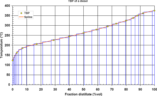 Figure 1: The TBP curve of example smoothed and cut into evenly-spaced temperature intervals.
In a second step, the characterization procedure is illustrated:
Once the petroleum mixture has been cut into pseudo-components, as shown in figure 1, each of the pseudo-component must be characterized for further calculation.
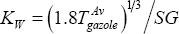
First, the average value of KW must be determined, as:
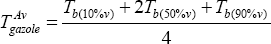
The average specific gravity, SG, is given (SG = 0.81130), but the average temperature is not known. It is computed from
Interpolating the curve, one can take:
| % volume | Tb (°C) |
|---|---|
| 10 | 188 |
| 50 | 258 |
| 90 | 353 |
Which yields:  = 264°C
And therefore:  =12.19 (rather paraffinic)
Using 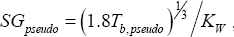 , where this time
  is the normal boiling temperature of the pseudo-component, the density of each of these components can be calculated (Table 3).
Before any calculation can be performed, the volume fractions must be converted into molar fractions. This requires the knowledge of the molecular masses. As an example, the method by Twu is used in Table 3.
| Pseudos | Tb Pseudos | Density | MW | % mol | Tc | Pc |
|---|---|---|---|---|---|---|
| °C | (kg/kmol) | (K) | (kPa) | |||
| Pseudo1 | 128 | 0.7360 | 114.8 | 0.0044 | 1.08% | 580.5 |
| Pseudo2 | 138 | 0.7420 | 120.1 | 0.0044 | 1.08% | 591.0 |
| Pseudo3 | 148 | 0.7480 | 125.6 | 0.0046 | 1.12% | 601.4 |
| Pseudo4 | 158 | 0.7539 | 131.2 | 0.0052 | 1.27% | 611.7 |
| Pseudo5 | 168 | 0.7596 | 136.9 | 0.0069 | 1.67% | 622.0 |
| Pseudo6 | 178 | 0.7653 | 142.8 | 0.0111 | 2.69% | 632.2 |
| Pseudo7 | 188 | 0.7710 | 148.9 | 0.0179 | 4.33% | 642.3 |
| Pseudo8 | 198 | 0.7765 | 155.0 | 0.0263 | 6.37% | 652.3 |
| Pseudo9 | 208 | 0.7819 | 161.4 | 0.0299 | 7.25% | 662.2 |
| Pseudo10 | 218 | 0.7873 | 167.8 | 0.0278 | 6.74% | 672.1 |
| Pseudo11 | 228 | 0.7926 | 174.5 | 0.0277 | 6.72% | 681.8 |
| Pseudo12 | 238 | 0.7979 | 181.3 | 0.0269 | 6.52% | 691.5 |
| Pseudo13 | 248 | 0.8030 | 188.3 | 0.0244 | 5.90% | 701.1 |
| Pseudo14 | 258 | 0.8081 | 195.4 | 0.0224 | 5.43% | 710.7 |
| Pseudo15 | 268 | 0.8132 | 202.7 | 0.0212 | 5.15% | 720.1 |
| Pseudo16 | 278 | 0.8182 | 210.2 | 0.0206 | 4.98% | 729.5 |
| Pseudo17 | 288 | 0.8231 | 217.9 | 0.0188 | 4.56% | 738.9 |
| Pseudo18 | 298 | 0.8279 | 225.8 | 0.0159 | 3.85% | 748.2 |
| Pseudo19 | 308 | 0.8327 | 233.9 | 0.0157 | 3.80% | 757.4 |
| Pseudo20 | 318 | 0.8375 | 242.2 | 0.0163 | 3.95% | 766.5 |
| Pseudo21 | 328 | 0.8422 | 250.8 | 0.0133 | 3.23% | 775.6 |
| Pseudo22 | 338 | 0.8468 | 259.5 | 0.009 | 2.17% | 784.7 |
| Pseudo23 | 348 | 0.8514 | 268.6 | 0.0081 | 1.97% | 793.7 |
| Pseudo24 | 358 | 0.8560 | 277.8 | 0.0111 | 2.69% | 802.7 |
| Pseudo25 | 368 | 0.8605 | 287.3 | 0.018 | 4.36% | 811.6 |
| Pseudo26 | 374 | 0.8631 | 293.2 | 0.0046 | 1.11% | 817.0 |
Comparison of the methods available for characterization:
In order to compare the various methods that exist a single component was taken (normal boiling temperature = 348 K and specific gravity 0.8479), and the characteristic properties calculated in table 4:
| MW (kg/kmol) | Tc (K) | Pc (kPa) | Vc (cm3/mol) | Zc (-) | |
|---|---|---|---|---|---|
| Twu [1] | 77.7 | 553.7 | 4745.9 | 277.1 | 0.286 |
| Cavett and Simsci [2] | 544.0 | 4258.9 | 291.0 | 0.274 | |
| Lee Kesler [3] | 77.8 | 550.3 | 4743.0 | 262.2 | 0.272 |
| Winn and Mobil + Hall-Yarborough[4] | 72.7 | 552.5 | 5248.7 | 246.0 | 0.281 |
| Riazi and Daubert 1[5] | 75.0 | 562.4 | 5001.5 | 268.1 | 0.287 |
| Riazi and Daubert 2 = API method[6] | 555.2 | 4338.1 | 291.1 | 0.274 |
We can see that all methods give similar results. This is so because the cut is a light one. In order to compare the various methods for heavy compounds a single component was taken (normal boiling temperature = 1165.35 K and specific gravity 1.045), and the characteristic properties calculated in table 5:
| MW (kg/kmol) | Tc (K) | Pc (kPa) | Vc (cm3/mol) | Zc (-) | |
|---|---|---|---|---|---|
| Twu [1] | 1663.1 | 1270.7 | 476.4 | 2858.2 | 0.129 |
| Cavett and Simsci [2] | 1320.4 | 4925.6 | -194.7 | -0.087 | |
| Lee Kesler [3] | 957.7 | 1220.3 | 234.1 | 5395.5 | 0.125 |
| Winn and Mobil + Hall-Yarborough[4] | 1163.0 | 1269.2 | 536.0 | 5050.8 | 0.257 |
| Riazi and Daubert 1[5] | 861.8 | 1234.8 | 496.5 | 3359.9 | 0.162 |
| Riazi and Daubert 2 = API method[6] | 1178.7 | 615.7 | 16604.9 | 1.043 |
The component chosen is rather heavy in order to stress that the differences may be large for such components. The method by Cavett and Simsci should clearly be avoided in that case (negative vc). The API recommended method by Riaizi and Daubert also provides a critical compressibility factor that is not realistic. Among the most realistic values, that proposed by Twu is probably most reasonable, because it is based on the extrapolation of the well-known behaviour of n-alkanes.
References
[1] TWU C.H., An internally consistent correlation for predicting the critical properties and molecular weights of petroleum and coal-tar liquids, Fluid Phase Equilibria, 1984, 16, n°2, p. 137-150. http://dx.doi.org/10.1016/0378-3812(84)85027-X
[2] CAVETT R.H., Physical Data for Distillation Calculations- Vapor-Liquid Equilibria, 1962.
[3] KESLER M.G., LEE B.I., Improve prediction of enthalpy of fractions, Hydrocarbon Processing, 1976, 55, p. 153-158.
[4] WINN F.W., Physical Properties by Nomogram, Petroleum Refiner, 1957, 36, p. 157-159.
[5] RIAZI M.R., DAUBERT T.E., Simplify property predictions, Hydrocarbon Processing, 1980, 59, n°3, p. 115-116.
[6] RIAZI M.R., Characterization and Properties of Petroleum Fluids, American Society for Testing and Materials, Philadelphia, 2005.