Chapter 3:
From Components
to Models
Abstract
Read the abstractTable of contents
See the table of contentsList of examples
- 3-1: Vapour pressure predictions of methane using different formulas
- 3-2: Quality evaluation of molar volume correlations
- 3-3: Evaluation of the ideal gas heat capacity equations for n-pentane
- 3-4: Quality evaluation of vapourisation enthalpy correlations
- 3-5: Comparison of second virial coefficient calculation methods
- 3-6: Comparison of critical points and acentric factor from different databases
- 3-7: Use of the group contribution methods of Joback and Gani
- 3.8: Diesel fuel characterization
- 3.9: Vapour pressures of di-alcohols
- 3.10: Find the parameters to fit the vapour pressure of ethyl oleate
- 3.11: Fitting of BIP coefficients for the mixture water + MEA with the NRTL model
- 3.12: Separation of n-butane from 1,3 butadiene at 333.15K using vapour-liquid equilibrium
- 3.13: Draw the heteroazeotropic isothermal phase diagram of the binary mixture of water and butanol at 373.15 K
- 3.14: Isothermal phase diagram using the Flory Huggins activity coefficient model
- 3.15: Use of an equation of state for pure component vapour pressure calculations
Example 3-14: Draw the isothermal phase diagram of the binary mixture of hexane + benzene with the Flory-Huggins activity coefficient model
The Flory-Huggins method is rather convenient as it is fully predictive (no binary interaction parameter to fit) and rather simple to use. It describes both enthalpic non-ideal behaviour, through the regular solution expression, and entropic deviations using the Flory term. It is not very precise, but provides a good indication regarding trends. In the example proposed here, it is applied to the binary system n-hexane (1) + benzene (2)
Analysis:
The Flory-Hugging activity coefficient model requires two pure component parameters for each component: the molar volume in the liquid phase and the solubility parameter. The molar volume can be calculated from the molar density which should be explained using DIPPR correlation (often, the value at 25°C is used, but this may be an improvement):
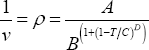
The calculation of the phase behaviour also requires to know the vapour pressure behaviour. In this work, the DIPPR correlation is used:
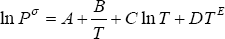
For both components, all of the parameters are found in the DIPPR database:
| DIPPR Density Coef. (Pa) | ||||
|---|---|---|---|---|
| A | B | C | D | |
| n-hexane | 0.70824 | 0.26411 | 507.6 | 0.27537 |
| Benzene | 1.0259 | 0.26666 | 562.05 | 0.28394 |
| Solub param | DIPPR Psat Coef. (Pa) | |||||
|---|---|---|---|---|---|---|
| (Pa^1/2) | A | B | C | D | E | |
| n-hexane | 1487 | 104.65 | -6995.5 | -12.702 | 1.2381E-05 | 2 |
| Benzene | 1874 | 83.107 | -6486.2 | -9.2194 | 6.9844E-06 | 2 |
Solution:
See complete results in file (xls):
Some help on nomenclature and tips to use this file can be found here.
All calculations are available in the “FloryHuggins” sheet. The calculations are performed as follows:
- the activity coefficient are calculated as a function of the liquid phase molar fractions (columns G to J in the excel sheet)
- The partial pressures (columns E and F) are then easily calculated
- The total pressure is the sum of the partial pressures (column D).
- From the partial pressure and the total pressure, the vapour phase molar fractions are found (column B)
In a last sheet, called “Data”, some experimental data have been collected. Figure 1 shows the good agreement between these data and the prediction of the model.
 Figure 1: comparison of predicted with experimental behaviour using the Flory-Huggins model on the n-hexane + benzene mixture at 328.15K.