Chapter 3:
From Components
to Models
Abstract
Read the abstractTable of contents
See the table of contentsList of examples
- 3-1: Vapour pressure predictions of methane using different formulas
- 3-2: Quality evaluation of molar volume correlations
- 3-3: Evaluation of the ideal gas heat capacity equations for n-pentane
- 3-4: Quality evaluation of vapourisation enthalpy correlations
- 3-5: Comparison of second virial coefficient calculation methods
- 3-6: Comparison of critical points and acentric factor from different databases
- 3-7: Use of the group contribution methods of Joback and Gani
- 3.8: Diesel fuel characterization
- 3.9: Vapour pressures of di-alcohols
- 3.10: Find the parameters to fit the vapour pressure of ethyl oleate
- 3.11: Fitting of BIP coefficients for the mixture water + MEA with the NRTL model
- 3.12: Separation of n-butane from 1,3 butadiene at 333.15K using vapour-liquid equilibrium
- 3.13: Draw the heteroazeotropic isothermal phase diagram of the binary mixture of water and butanol at 373.15 K
- 3.14: Isothermal phase diagram using the Flory Huggins activity coefficient model
- 3.15: Use of an equation of state for pure component vapour pressure calculations
Example 3-13: Draw the isothermal phase diagram of the binary mixture of water and butanol at 373.15 K
The water (1) + 1-butanol (2) mixture can be modelled using the Margules activity coefficient representation with following parameters (water and butanol as both solvents), with the following parameters: A12=1.3863 and A21=3.0445(dimensionless).
The vapour pressures of the pure components are:
Pσ1 = 101.261 kPa
Pσ2 = 52.098 kPa
Analysis:
A complete isothermal phase diagram for a binary system must be constructed. Therefore, no feed composition is required. Only phase equilibria need to be calculated. However, we do not know in advance what type of phase equilibria may occur, and all possibilities must be checked.
Vapour - Liquid equilibrium always occurs if the temperature is between the triple point temperature and the critical temperature of any one of the components.
The system contains highly polar components, which means that a strongly non-ideal system is expected. Pressures are low, so an activity coefficient model is acceptable. In this example, the Margules equation is used:
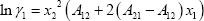
and:
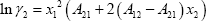
With the parameters provided, we find:
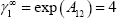
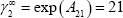
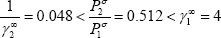
It is also possible to state that the vapour-liquid equilibrium will present an azeotropic behaviour, using the criterion defined in the textbook:
Solution:
See complete results in file (xls):
Some help on nomenclature and tips to use this file can be found here.
All calculations are available in the “Margules” sheet. The calculations are performed as follows:
- the activity coefficient are calculated as a function of the liquid phase molar fractions (columns G/I and H/J in the excel sheet)
- The partial pressures (columns E and F) are then easily calculated according to the Raoult’s law
- The total pressure is the sum of the partial pressures (column D)
- From the partial pressure and the total pressure, the vapour phase molar fractions are easily found (column B).
With all these results, we should draw the phase diagram (cf. Figure 1). At this point, it can be noticed that the calculated isothermal phase diagram features a non-physical behaviour: the bubble pressures (x vs P) has two maxima that are not azeotropic, and the dew pressure (y vs P) shows a loop.
 Figure 1: First drawing of the water + 1-butanol phase diagram
When this kind of phase diagram is found, the reader should immediately consider that in reality the system features a liquid-liquid phase split that the calculation mode cannot make visible. At the crossing of the two dew lines, it can be stated that the vapour phase is in equilibrium with two distinct liquid phases. This means that at higher pressures, a liquid-liquid phase split exists.
In order to better understand this phase diagram, we should perform a stability analysis. This consists in examining the Gibbs energy of the liquid and the vapour phases.
The liquid Gibbs energy is the sum of the ideal Gibbs energy of mixing and the excess Gibbs energy determined from the activity model. To simplify the calculation, we have assumed the liquid Gibbs energy references equal to 0 for both components ( =
= =0):
=0):
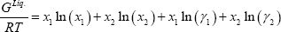
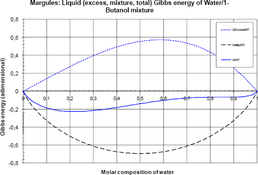 Figure 2 Liquid (excess, mixture and total) Gibbs energy as a function of the composition
The ideal Gibbs energy of mixing gives the lower symmetric curve and the excess Gibbs energy a positive asymmetric one. The sum is asymmetric and negative.
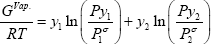
The vapour Gibbs energy is written assuming that the vapour phase is ideal due to the low total pressure level.
Note that since we have chosen the pure component liquid Gibbs energies for both components to be zero at the mixture pressure and temperature conditions, their vapour Gibbs energies are not zero. We now need to calculate the Gibbs energy of the vapour in the reference state for both compounds. These values are calculated from the liquid-vapour equilibrium of pure compound:
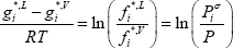
Hence ( =0)
=0)
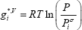
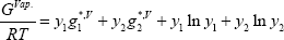
with  the vapour pressure of the pure compound. We can see that assuming a null reference state of the liquid yields a reference state of the vapour related to the vapour pressure. So, the Gibbs energy of the vapour phase should be calculated as:
Now, we should carry on the analysis of the Gibbs energy based on the comparison of the liquid and the vapour curves. Let us start at low pressure (40kPa). Figure 3a shows the Gibbs energies and figure 3b the Pxy diagram.
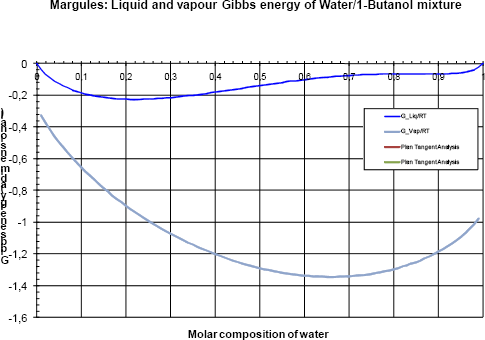 Figure 3a Gibbs analysis at 40 kPa
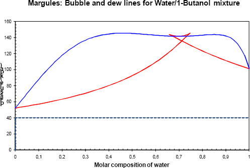 Figure 3b Phase diagram of the binary with a pressure of 40 kPa.
The Gibbs energy of the vapour phase is lower than the Gibbs energy of the liquid phase and only the vapour phase is stable.
For a slightly higher pressure (80 kPa), the Gibbs energy of the liquid phase and of the vapour phase cross (figure 4a). For low water concentrations (below 0.08), the liquid phase is stable. For high water concentration (above 0.4) the vapour phase is the most stable. Between these two regions (i.e. in the [0.08; 0.4] range of water) the mixture composed of the two phases is more stable than each one individually (tangent plane criterion) and a vapour – liquid equilibrium is observed (figure 4b).
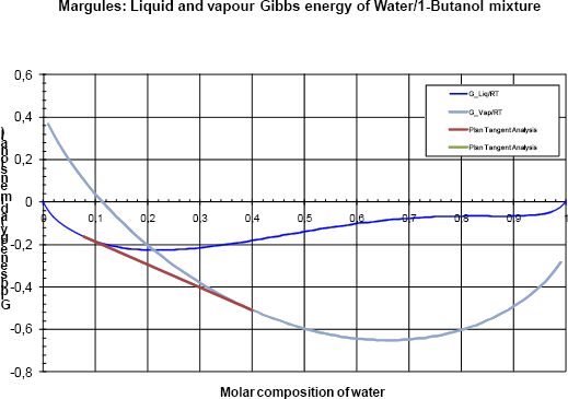 Figure 4a Gibbs analyses at 80 kPa
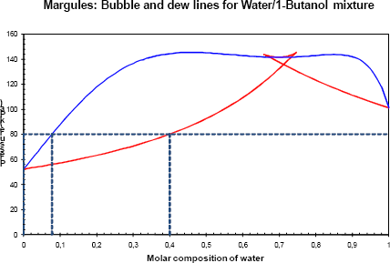 Figure 4b Phase diagram of the binary with a pressure of 80 kPa.
The analysis is now carried out at (P=120 kPa) (figures 5a and 5b). It now becomes clear how two vapour- liquid zones appear (two tangent plane regions) at the same pressure, one at low water concentration (between 0.21 and 0.65 molar fraction) and one at high water concentration (between 0.82 and 0.98 molar fraction).
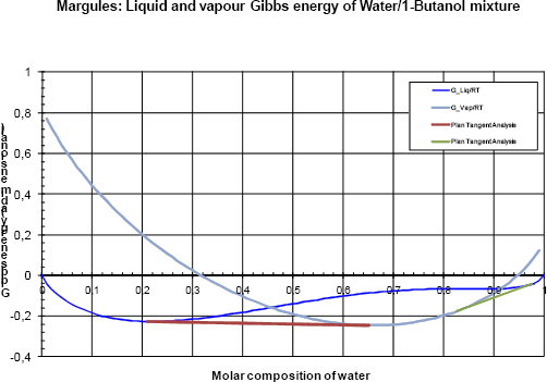 Figure 5a Gibbs analyses at 120 kPa
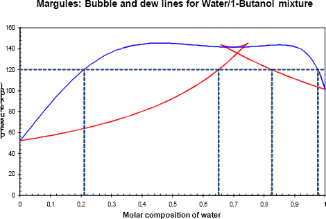 Figure 5b Phase diagram of the binary with a pressure of 120 kPa.
For a pressure equal to 136 kPa (the crossing of the two dew lines) figure 6a shows that the two tangent planes merge and are equal to the tangent to the Gibbs energy of the vapour phase. It can be stated that the vapour phase is in equilibrium with two distinct liquid phases. This is the three phase pressure of the system.
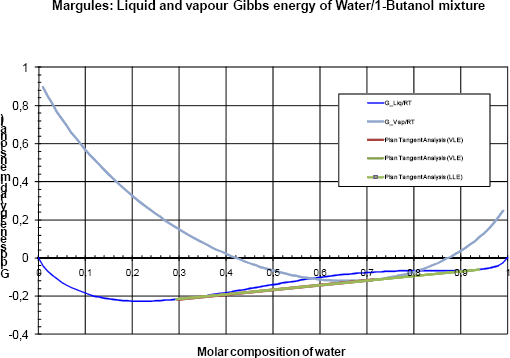 Figure 6a Gibbs analyses at 136 kPa
 Figure 6b Phase diagram of the binary with a pressure of 136 kPa.
Finally, for higher pressures (e.g. P = 160 kPa, as illustrated in figure 7), the liquid phases are more stable than the vapour. For a molar fraction of water less than 0.3 or greater than 0.9, only one liquid phase is stable and in the range of [0.3 ; 0.9], a liquid-liquid phase split is observed.
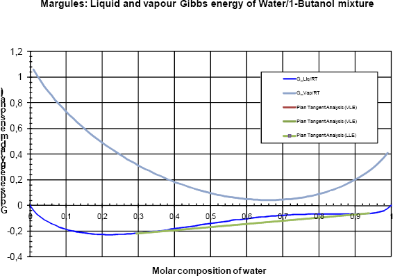 Figure 7 Gibbs analyses at 160 kPa
Figure 8 shows at 373.15 K the final isothermal hetero-azeotropic phase diagram of the water + 1 butanol mixture. Note that the liquid-liquid region is presented by a vertical slice. This is a result of the assumption that the activity coefficient is independent of pressure. As a first approximation, it is a good solution, but the graph cannot be extended to pressures larger than 1 MPa.
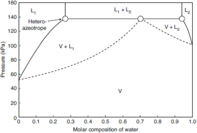 Figure 8: Pxy diagram for the water + 1-butanol mixture at 100 °C (373.15 K).